Moon Temp — Project Overview

Hardware build, measurement methodology, and analysis pipeline for the Moon Temp experiment.

Rooster.ninja — Moon Temp

Moon Temp — Experiment Overview

An outdoor instrument array built to test whether moonlight produces a measurable thermal signature detectable by extremely sensitive NTC thermistors.

1. Introduction & Hypothesis

This experiment addresses a deceptively simple question: can moonlight produce a detectable temperature differential at the surface of a sensitive thermistor array?

Rather than attempting a direct measurement of moonlight intensity, the experiment uses a differential approach: two sensors exposed to moonlight are compared against one sensor placed in the moon’s shadow. If moonlight has any thermal effect on the sensors, the illuminated and shaded channels should diverge in a sustained, systematic manner following exposure onset.

Hypothesis

	Statement
H₀ (Null)	Moonlight has no measurable effect on raw ADC counts acquired from the thermistor array. Any observed differences between illuminated and shaded sensors are attributable to sensor noise and ambient environmental drift.
H₁ (Alternate)	Moonlight induces a statistically detectable differential thermal response. Illuminated and shaded sensors diverge in a sustained, systematic manner during a moon event.

The experiment is conducted during full or near-full moon events, when moonlight is sufficient to produce a measurable effect at the sensor surface. The null hypothesis is evaluated independently for each event.

2. Test Rig & Sensor Layout

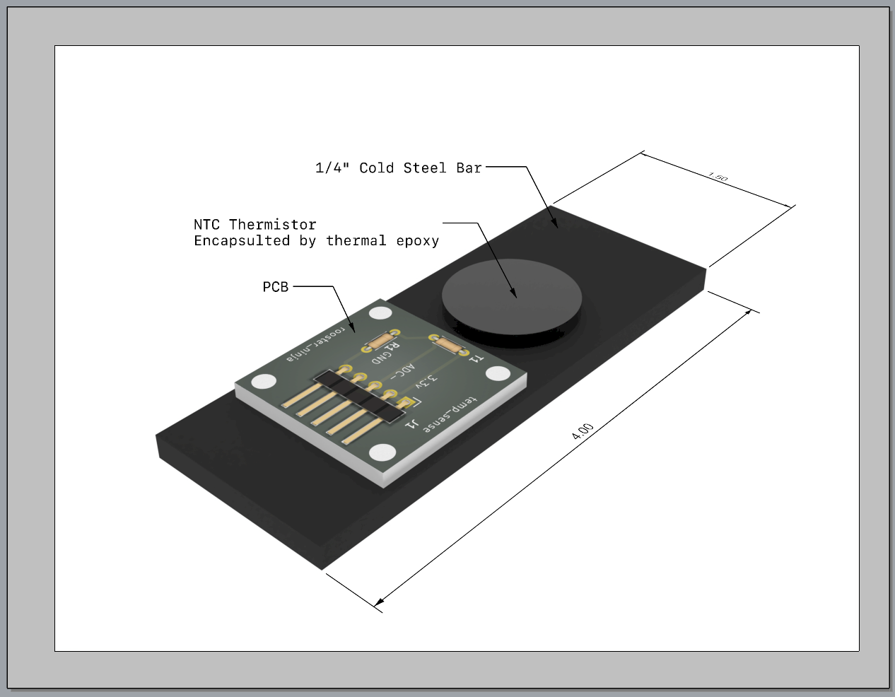
The test rig holds three MF58 10 kΩ NTC thermistors, evenly spaced along a rigid mount. Each sensor is thermally isolated from the mounting structure via foam insulation to minimise conductive heat transfer from the structure itself.

Channel	Designation	Lunar Exposure
ADC0	Sensor 0	Moonlit — primary illuminated reference
ADC1	Sensor 1	Moonlit — secondary illuminated reference
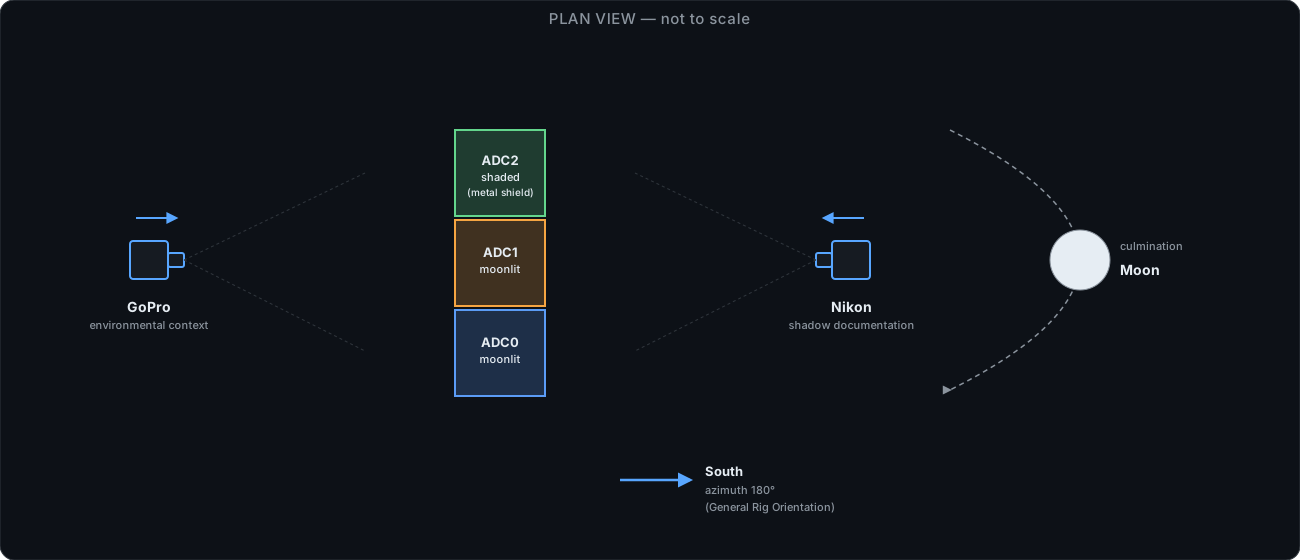
ADC2	Sensor 2	Shaded — blocked from direct moonlight by a metal shield

ADC0 and ADC1 serve as paired moonlit reference channels. ADC2 is the experimental shaded channel. The metal shield configuration — and any additional insulation applied to it — is a methodological variable noted per run session.

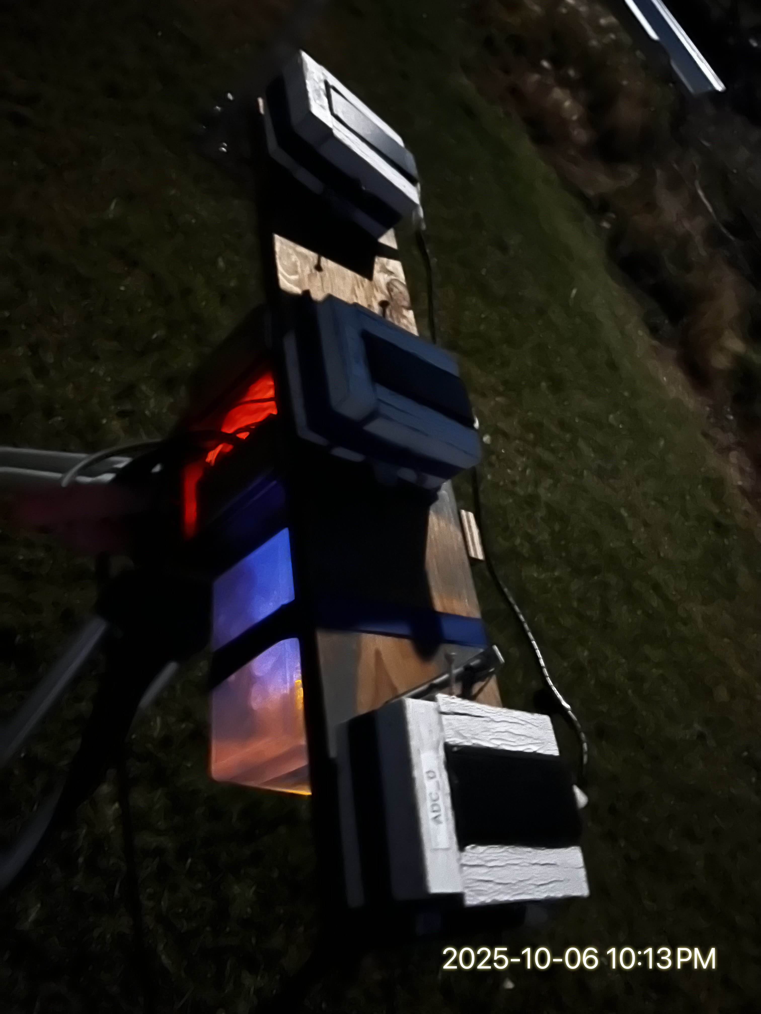
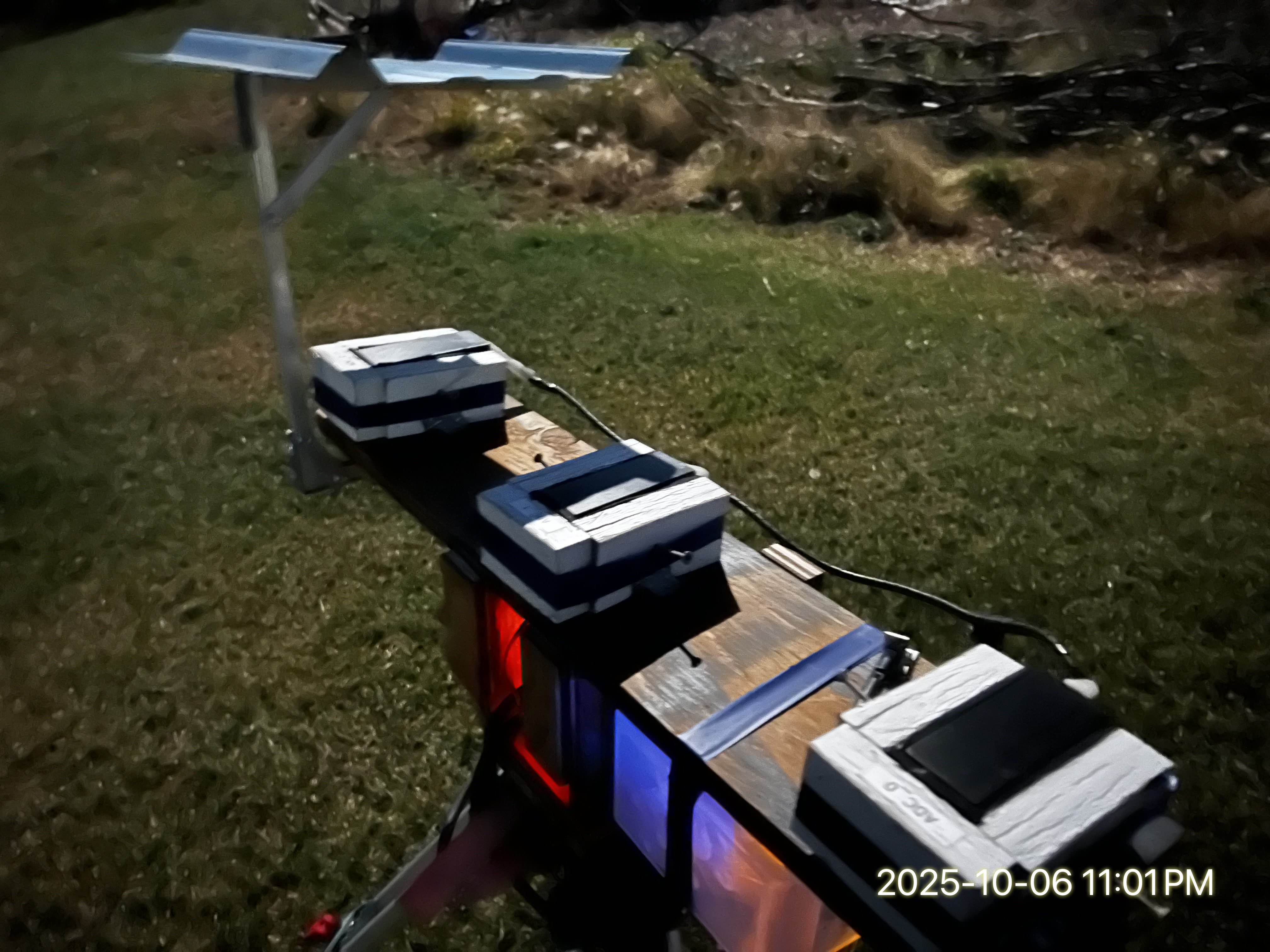
NTC thermistor assembly — sensor epoxied into a steel bar thermal mass

Field Deployment

Deployed rig during a moon event — three sensor enclosures mounted on the rig with the metal shadow shield visible at top. The red LED indicates the power supply; blue LED indicates the ESP32-C3 WiFi/MQTT activity.

Sensor rig during a Harvest SuperMoon event — close view showing ADC_0 label and sensor enclosures Sensor rig during a moon event — full view showing all three sensor enclosures and metal shadow shield

3. Hardware

Measurement Circuit

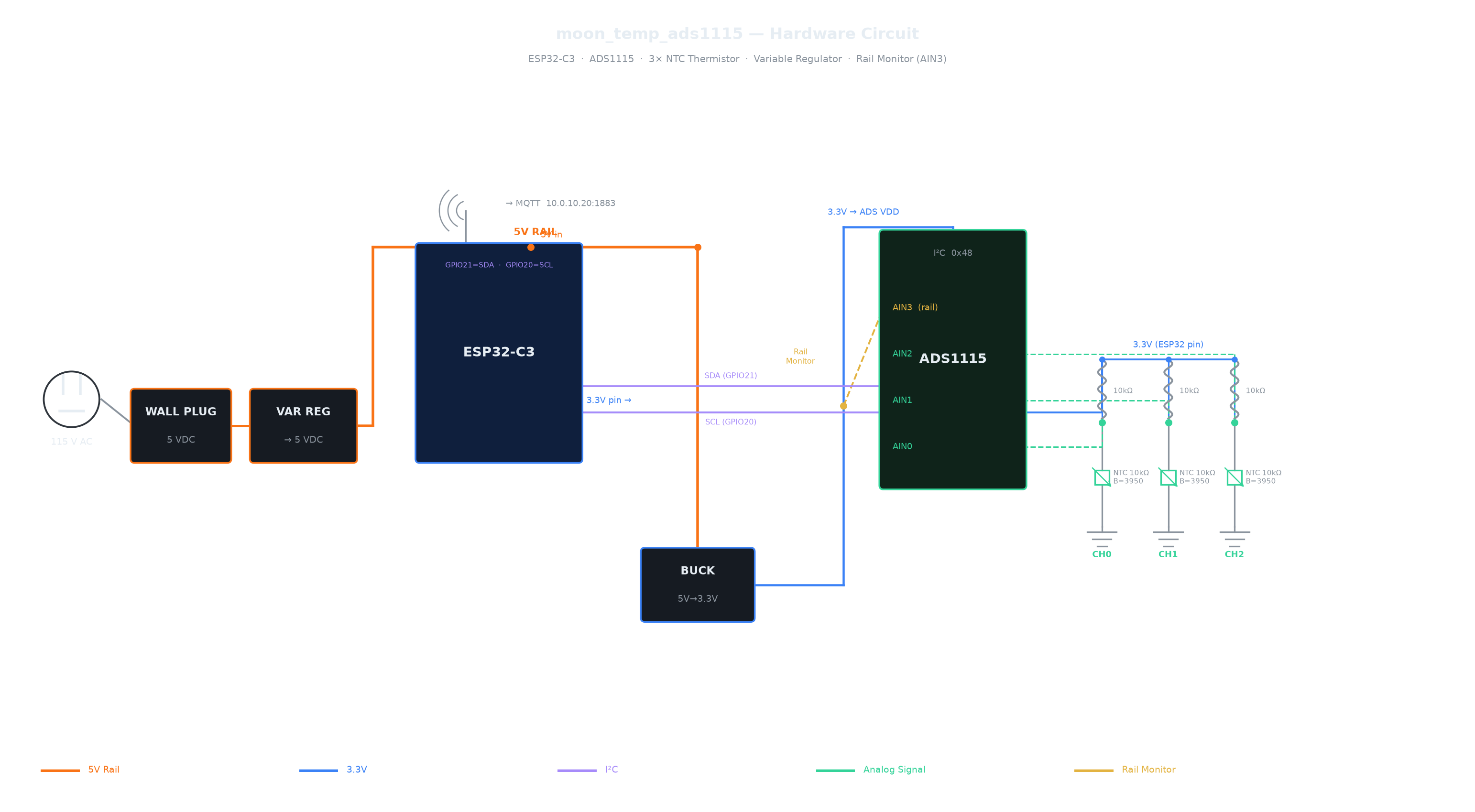
Each sensor channel uses a voltage divider configuration. A fixed 10 kΩ series resistor is placed between the supply rail and an ADS1115 ADC input; the NTC thermistor connects from that input to ground. The midpoint voltage — which varies with thermistor resistance and therefore with temperature — is digitised by the ADC.

A fourth ADC input (AIN3) monitors the supply rail voltage \(V_\text{rail}\) directly. This measured value is used during temperature conversion in place of a fixed voltage assumption, correcting for rail fluctuations.

Moon Temp circuit diagram — voltage divider, ADS1115, ESP32-C3 (placeholder; official design files to follow)

Component Specifications

Component	Specification
Thermistors	3× MF58 10 kΩ NTC, \(B = 3950\,\text{K}\), \(R_0 = 10\,\text{k}\Omega\) @ 25 °C
Series resistor	10 kΩ fixed (per channel)
ADC	ADS1115, 16-bit, I²C 0x48, PGA ±4.096 V, 128 SPS
Microcontroller	ESP32-C3; I²C SDA → GPIO 21, SCL → GPIO 20
Resolution	~55 m°C per ADC count at 26 °C

Power Chain

Stage	Detail
Mains	115 V AC → 5 VDC wall adapter
Variable regulator	Adjustable output → 5 V rail
ESP32-C3	Powered directly from 5 V rail
Buck converter	5 V → 3.3 V dedicated supply for ADS1115 V_DD
Rail monitor	ADS1115 AIN3 wired to ADS1115 V_DD → logged as `v_rail`

Hardware Photos

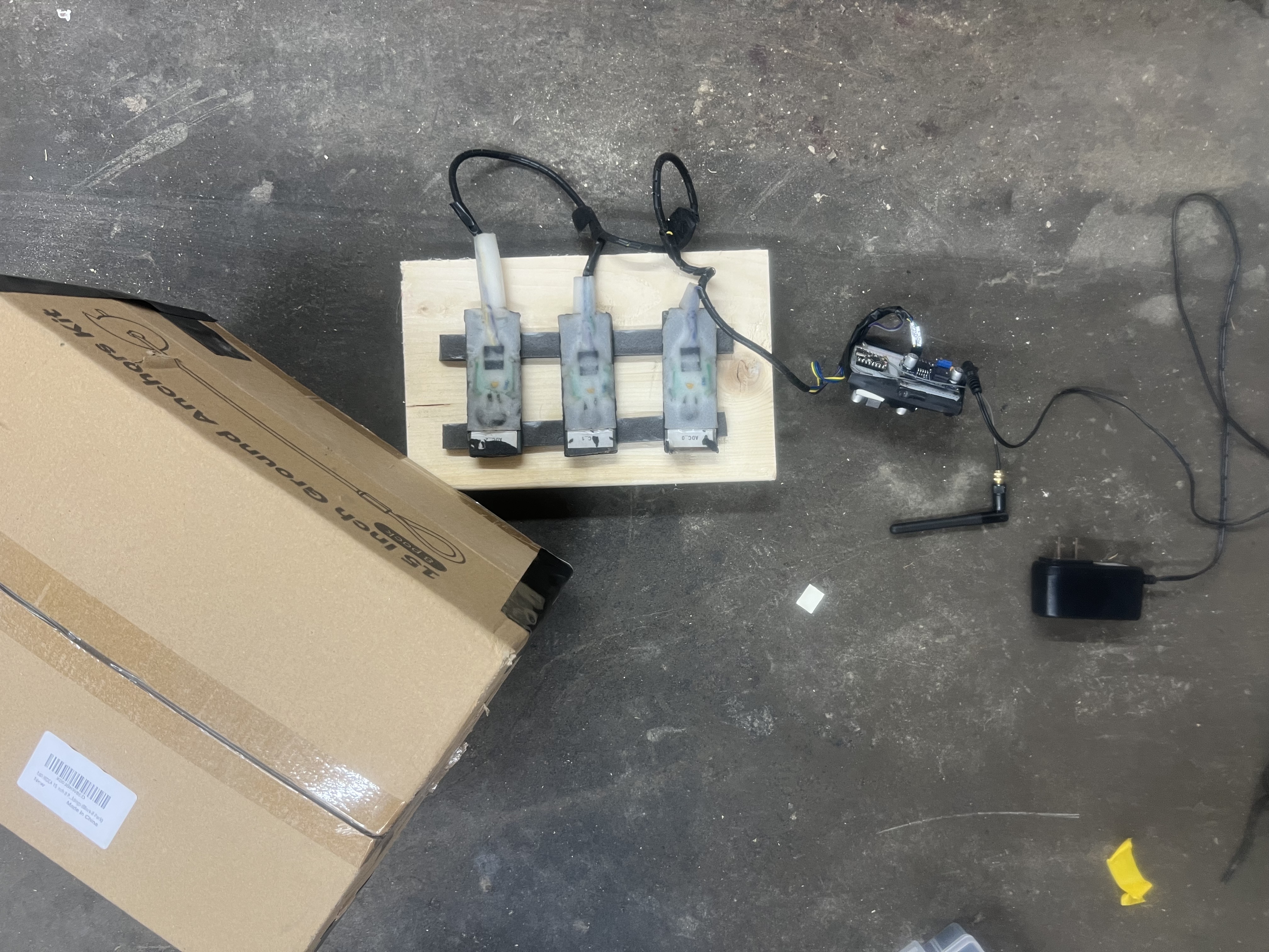
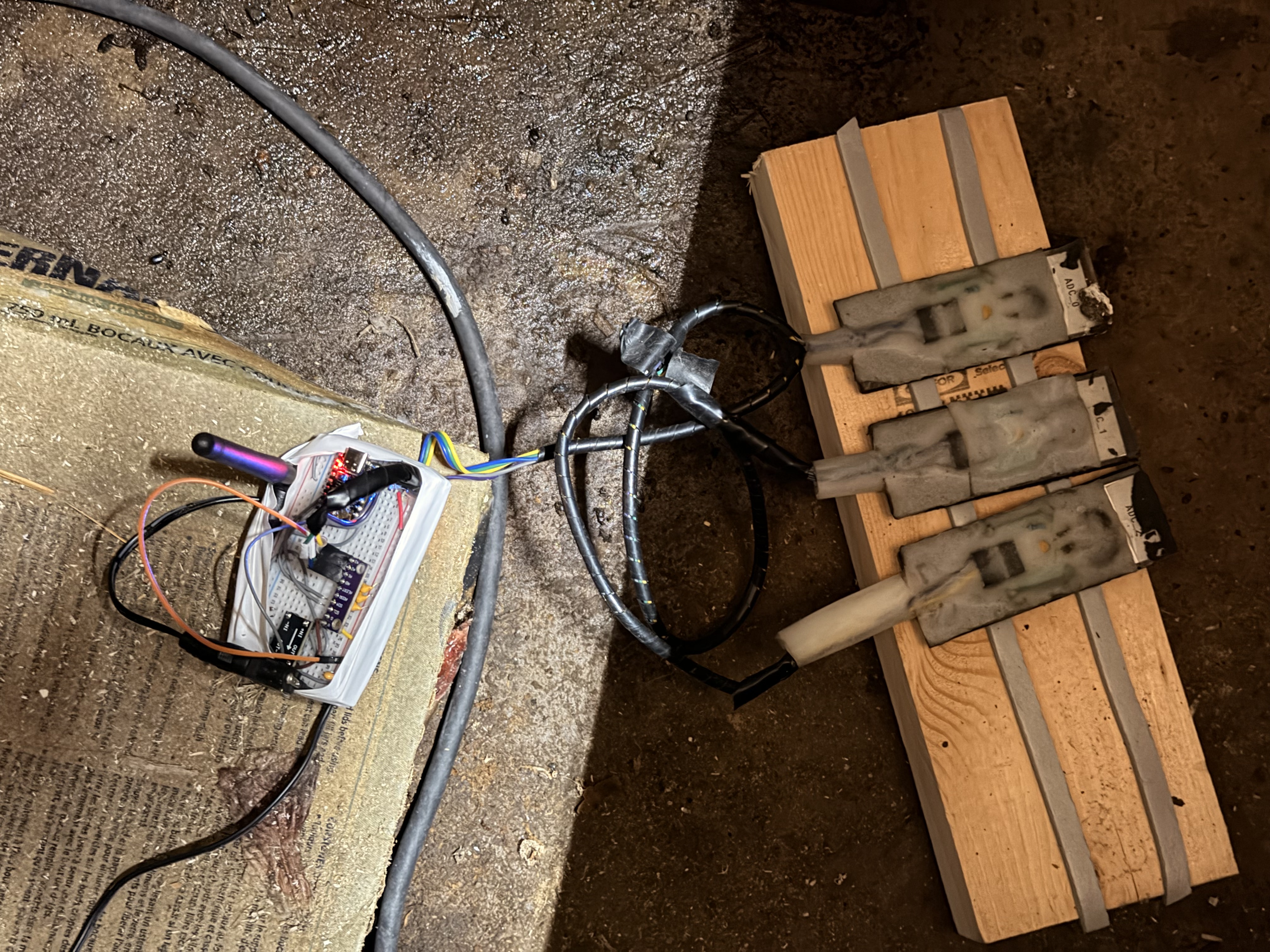
Photos taken during the calibration phase prior to field deployment.

Three NTC sensor assemblies on wooden mount with ESP32-C3 — bench setup during calibration ESP32-C3 breadboard and three NTC sensor assemblies deployed in static thermal chamber during calibration

4. Software & Data Collection

Firmware

The ESP32-C3 runs a Rust/Embassy async firmware stack. On receipt of a senddata MQTT request, the firmware polls all four ADS1115 channels (ADC0–ADC2 sensors + AIN3 rail monitor), applies per-channel offset corrections stored in flash, and publishes a JSON payload to the broker.

Each published value is the average of 64 samples at 128 SPS (~2.3 seconds of acquisition per publish), which suppresses single-sample noise spikes observed in earlier single-sample builds.

Logger

Host-side logging software (moon_temp_logger, Rust) issues senddata requests at a configurable interval (default: 60 seconds) and writes two daily rolling CSV files:

File	Columns
Raw	`timestamp, adc0, adc1, adc2, v_rail`
Converted	same + `t0_c, t1_c, t2_c` (degrees Celsius)

Data is written to /mnt/nas/rooster/moon-temp-logs/ as daily rolling CSV files. During live moon events, the /moon-temp-notes session capture procedure is used to record real-time observations alongside the automated data stream.

Deployment — Local Server (DebServ)

The logger runs as a systemd service on the home server (deb-serv-incus, 10.0.10.20). It connects to the local MQTT broker and subscribes to the device data topic.

Parameter	Value
MQTT broker	`10.0.10.20:1883`
Sensor ID	`moon-temp-001`
Subscribed topic	`moon-temp-001/data`
Raw logs	`/mnt/nas/rooster/moon-temp-logs/raw_logs`
Converted logs	`/mnt/nas/rooster/moon-temp-logs/converted_logs`
Request interval	60 s

Minute synchronisation: On startup, the logger calculates the time remaining until the next whole-minute boundary (via NTP, accuracy ~10–50 ms) and delays the first senddata request until that boundary. Subsequent requests fire at 60-second intervals from that aligned start. This ensures all data timestamps fall on whole UTC minutes, tightening synchronisation with the camera timelapse systems.

moon_temp_logger startup log — config, broker, sensor ID, NTP minute-sync

To restart the service and inspect startup logs:

sudo systemctl restart moon_temp_logger && sudo journalctl -u moon_temp_logger -n 10 --no-pager

Temperature Conversion Pipeline

Converted temperature files are produced on the logger host by applying the following four-step pipeline to each row.

Step 1 — ADC count → channel voltage

\[V_\text{out} = N_\text{ADC} \cdot \frac{V_\text{FSR}}{2^{15} - 1}, \qquad V_\text{FSR} = 4.096\,\text{V}\]

Step 2 — Rail voltage (AIN3 count → measured supply voltage, used in place of a nominal 3.3 V assumption)

\[V_\text{rail} = N_\text{rail} \cdot \frac{V_\text{FSR}}{2^{15} - 1}\]

Step 3 — Voltage divider → NTC resistance

Circuit topology: \(V_\text{rail} \to R_\text{fixed} \to V_\text{out} \to R_\text{NTC} \to \text{GND}\)

\[R_\text{NTC} = R_\text{fixed} \cdot \frac{V_\text{out}}{V_\text{rail} - V_\text{out}}, \qquad R_\text{fixed} = 10\,\text{k}\Omega\]

Step 4 — Beta equation → temperature

\[\frac{1}{T} = \frac{1}{T_0} + \frac{1}{B}\ln\!\left(\frac{R_\text{NTC}}{R_0}\right)\]

\[T_C = T - 273.15 \quad (°\text{C})\]

where \(T_0 = 298.15\,\text{K}\), \(B = 3950\,\text{K}\), \(R_0 = 10\,\text{k}\Omega\) (MF58 NTC datasheet values).

5. Camera Documentation

Two cameras document each moon event independently.

Camera	Position	Purpose	Interval
GoPro Hero 4	Behind rig	Environmental context — cloud cover, moon position, general scene conditions	1 min
Nikon DSLR	Front-facing	Shadow documentation — exact lunar shadow position on sensor array during event	1 min

Both cameras are set to a 1-minute capture interval and compiled to 30 FPS video (1 frame per 2 seconds of real time). This frame rate is consistent across both cameras, simplifying synchronisation during video production.

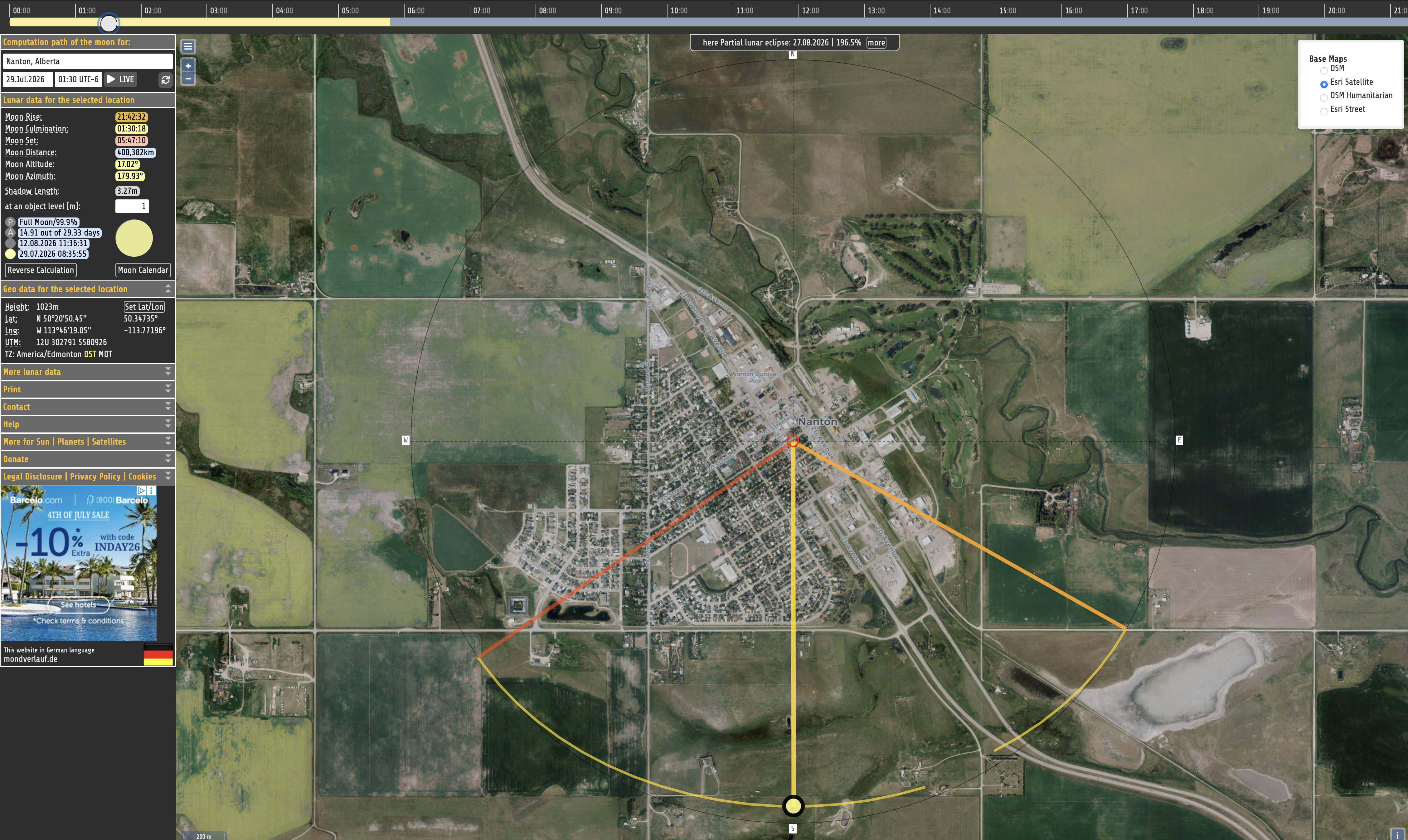
Moon events are planned using a lunar arc calculator to determine rise, culmination, set times, and shadow geometry for the observation site region.

Lunar arc planning tool — moon rise, path, and shadow arc for the observation site region

Time Synchronisation

Source	Accuracy	Method
GoPro	±1 minute	Start time set explicitly to match logger start timestamp
Nikon	±10 seconds	Timestamps are GPS-time-accurate; timelapse start depends on a manual button press
Logger	~10–50 ms (NTP)	NTP-synced; first `senddata` request aligned to next whole-minute boundary at startup

The Nikon shadow footage is post-processed into a timestamped video file and manually aligned to the data time series for side-by-side presentation in the event analysis.

6. Post-Analysis Pipeline

Each moon event is analysed in a dedicated Jupyter notebook. The analysis proceeds through the following stages:

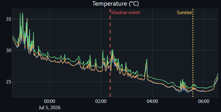
Data loading — Raw CSV imported; shadow event timestamp and analysis window defined (pre-shadow baseline through sunrise −1 hr).
Full session overview — Interactive time series of all three ADC channels and derived temperatures.
Difference signal construction — The mean of the illuminated reference channels is subtracted from the shaded channel:

\[\Delta = \text{ADC2} - \frac{\text{ADC0} + \text{ADC1}}{2}\]

This difference signal cancels shared environmental drift (ambient temperature variation, electrical noise) and isolates any moon-specific effect on the shaded sensor.

Pre-shadow baseline characterisation — Noise floor and inter-channel statistics computed over the pre-event window (calibrated noise floor: ±3 ADC counts).
Distribution comparison — Pre vs post-shadow delta histograms and box plots.
Rolling slope analysis — A 45-minute sliding window slope is computed over \(\Delta\) to detect sustained trend changes. Because sensor thermal mass acts as a low-pass filter, the analysis looks for a change in the rate of change of \(\Delta\) rather than an instantaneous step at shadow onset, and allows for a lag relative to the recorded event time.

Statistical Tests

Test	Purpose
Autocorrelation-corrected \(t\)-test	Compares pre- vs post-shadow slopes of \(\Delta\); adjusts for serial correlation via effective sample size \(n_\text{eff}\)
Segmented OLS with HC3 robust SE	Piecewise linear model fitted at shadow onset; primary test: interaction term (slope change); secondary: level-shift coefficient
Lag-1 autocorrelation correction	\(n_\text{eff} = n \cdot \dfrac{1 - r_1}{1 + r_1}\), where \(r_1\) is the lag-1 autocorrelation of the residuals

Sign convention: Higher ADC counts correspond to lower temperature — a cooler NTC thermistor has higher resistance, which raises the voltage divider midpoint voltage. The direction and magnitude of any divergence in \(\Delta\) is determined by the data.

Outcome

For each event, H₀ is either rejected (statistically significant slope change in \(\Delta\) at shadow onset) or failed to reject (no significant divergence detected). Results, data, and analysis notebooks are published to rooster.ninja.

Special Thanks

This project would not exist without the curiosity and encouragement of the following communities.

Man of Stone

Bitchute Channel

Aether Cosmology Discord

Join the Discord