import numpy as np
import matplotlib.pyplot as plt
import matplotlib.patches as mpatches
from matplotlib.ticker import MultipleLocator

BG      = "#0d0f12"
SURFACE = "#151820"
BORDER  = "#252a35"
ACCENT  = "#4fa3e0"
ACCENT2 = "#7ed6a0"
TEXT    = "#d8dce8"
MUTED   = "#6b7280"
HEADING = "#f0f4ff"
WARN    = "#f78c6c"
C3      = "#c792ea"

plt.rcParams.update({
    'figure.facecolor': BG, 'axes.facecolor': SURFACE,
    'axes.edgecolor': BORDER, 'axes.labelcolor': TEXT,
    'xtick.color': MUTED, 'ytick.color': MUTED,
    'text.color': TEXT, 'grid.color': BORDER,
    'grid.linewidth': 0.5, 'font.family': 'sans-serif', 'font.size': 11,
    'axes.spines.top': False, 'axes.spines.right': False,
})

CABLE_ELEC = 0.695   # m

# ── Calibration run data ──────────────────────────────────────────────────────
baseline_means  = [-6.877, -6.990, -6.890, -6.947, -6.999]
baseline_sigmas = [ 0.674,  0.884,  0.882,  0.650,  0.477]

iter1_means     = [-3.1125, -3.3078, -3.2223, -3.2039, -3.2977]
iter1_sigmas    = [ 0.4519,  0.4386,  0.4388,  0.4482,  0.4773]

iter2_means     = [0.6499, 0.6674, 0.6874]
iter2_sigmas    = [0.4758, 0.4671, 0.4729]

table_vals = [13430, 13264, 13089]
group_means = [np.mean(baseline_means), np.mean(iter1_means), np.mean(iter2_means)]
group_sigmas = [np.mean(baseline_sigmas), np.mean(iter1_sigmas), np.mean(iter2_sigmas)]SX1280 Hardware Ranging — Calibration
Project: Giga Ranger — GPS-independent distance measurement via SX1280 Time-of-Flight Hardware: LILYGO T3-S3 (ESP32-S3) · SX1280 @ 2.45 GHz · 13 dBi Yagi · 60 km fixed LOS link, Stubbornly Sovereign Alberta Method: Conducted (cabled) calibration — Wolf et al. (2019) §IV.A.1 + Semtech AN1200.29 Devices: Alpha (permanent master) · Chimp-001 (permanent slave) Calibration date: 2026-07-04 · Die temp: 31.3°C
| Parameter | Value |
|---|---|
| Spreading Factor | SF9 |
| Bandwidth | 1625 kHz |
CAL_TABLE[2][4] |
13089 |
| AN1200.29 default | 13430 |
| Total correction | −341 counts |
| Verification mean | +0.668 m |
| Cable electrical length | 0.695 m |
| Residual | −27 mm |
| CalibrationValue | 0 |
Theoretical accuracy at 60 km (calibration applied): ±0.47 m per exchange (1σ) · ±0.021 m averaged over 500 exchanges
1. Background
The SX1280 integrates a hardware Time-of-Flight ranging engine. The master transmits a ranging request; the slave responds after a fixed internal turnaround delay; the master measures the round-trip time and converts it to distance. The result is a 24-bit integer in units of c / (2 × BW × 2^SF) — for SF9/BW1625: 0.1803 m per count.
The SX1280 subtracts a nominal turnaround time internally, but each chip has a slightly different actual RX→TX switching delay. This systematic offset must be measured and corrected per board. The correction lives in Chimp-001’s RxTxDelay register — adjusted via a calibration table passed to startRanging().
In RadioLib 7.7.1, setRangingCalibration() does not exist. The calibration is applied by passing a custom 3×6 table (rows = BW, columns = SF5–SF10) to startRanging() on every exchange.
See Appendix A for a detailed explanation of why calibration lives on the slave (Chimp-001).
2. Hardware Setup
Devices
| Device | Role | Notes |
|---|---|---|
| Alpha | Permanent master (initiator) | LILYGO T3-S3 V1.3, SX1280 |
| Chimp-001 | Permanent slave (responder) | LILYGO T3-S3 V1.3, SX1280 |
Calibration signal chain
[Alpha] ── SMA ── [40 dB atten] ── [1 m RG-316 coax] ── [Chimp-001]TX power: −18 dBm (SX1280 minimum). With one 40 dB attenuator: −58 dBm at RX. No antenna fitted during calibration.
Reference cable
| Property | Value |
|---|---|
| Part | DigiKey J10302-ND — Amphenol RG-316 MIL-DTL-17 |
| Physical length | 1.000 m |
| Velocity factor | 0.695 (MIL-DTL-17 spec, confirmed from jacket markings) |
| Electrical length | 0.695 m (calibration target) |
Calibration rig — 2026-07-04
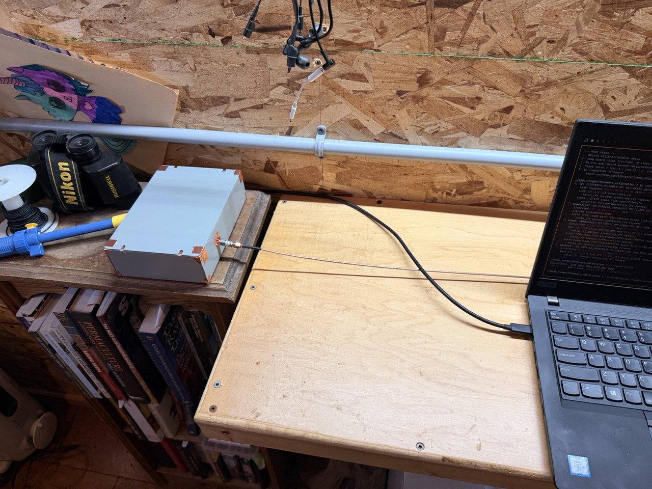
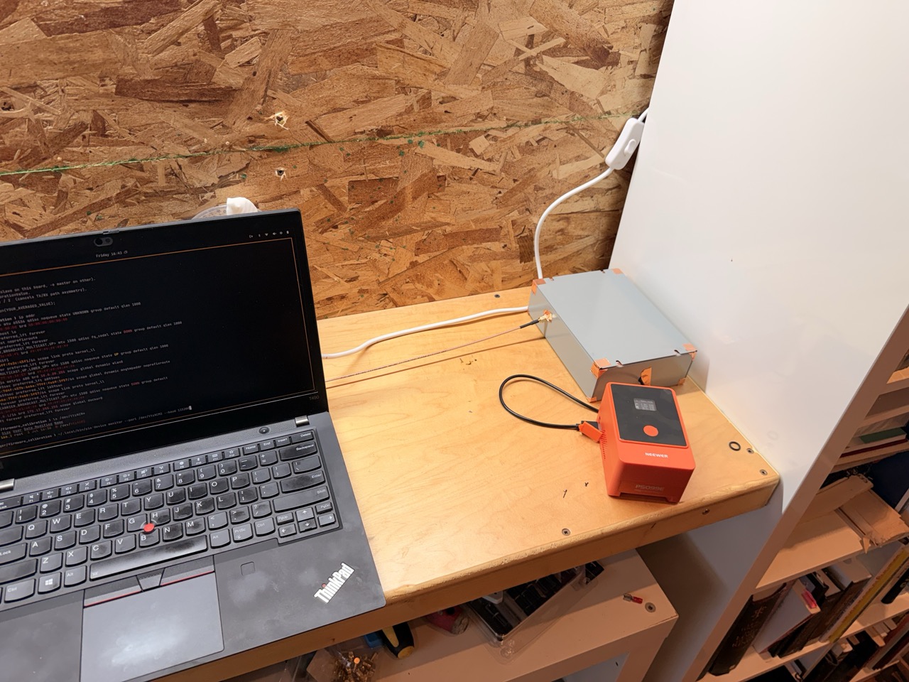
Figure 1 — Full setup: Alpha and Chimp-001 connected via 40 dB attenuator and 1 m RG-316 reference cable. RF enclosures sealed to reduce spurious coupling.
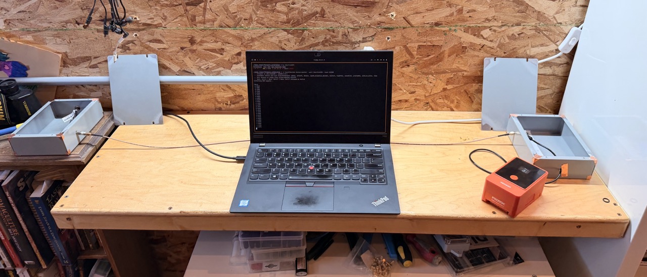
Figure 2 — Alpha (master)
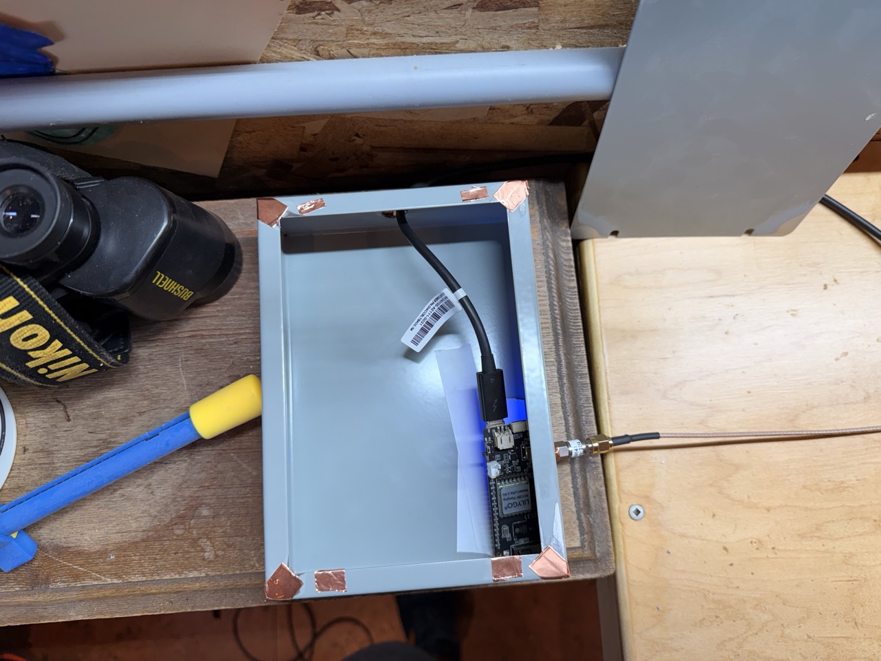
Figure 3 — Chimp-001 (slave)
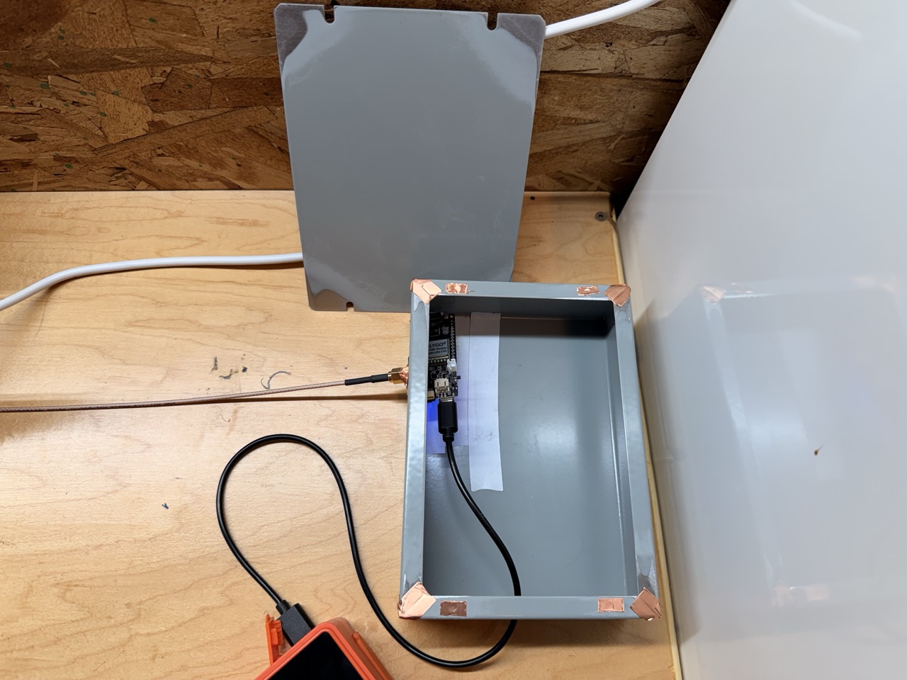
Figure 4 — Sealed enclosures during calibration run
3. Chimp Calibration Method
The Chimp Calibration method uses Alpha as the permanent master across all calibration runs. Only Chimp-001’s RxTxDelay register is corrected — its slave-mode delay is what Alpha measures.
Steps: 1. Flash Chimp-001 (-e slave), then Alpha (-e master) 2. Assemble the cabled signal chain; seal RF enclosures 3. Press SPACE on Alpha’s serial monitor to start a 500-exchange collection pass 4. Record Mean, CalibrationValue, and ESP32 die temp 5. Repeat 3–5 passes to establish a stable baseline mean 6. Adjust CAL_TABLE[2][4] by the CalibrationValue × empirical table rate 7. Reflash Alpha (Chimp-001 does not need reflashing — table is passed from Alpha at runtime) 8. Repeat until CalibrationValue ≈ 0 and Mean ≈ 0.695 m
Empirical table rate for SF9: ~0.0224 m per table count (measured from iteration 1 convergence). This is approximately half the SF10 rate (0.0456 m/count), consistent with the SF doubling relationship.
See Appendix B for a note on the AN1200.29 role-reversal averaging method and why it was not used here.
fig, axes = plt.subplots(1, 2, figsize=(14, 5))
fig.patch.set_facecolor(BG)

# ── Left: mean convergence per run ───────────────────────────────────────────
ax = axes[0]
all_means  = baseline_means + iter1_means + iter2_means
all_sigmas = baseline_sigmas + iter1_sigmas + iter2_sigmas
n = len(all_means)
x = np.arange(1, n + 1)

colours = ([ACCENT] * len(baseline_means) +
           [ACCENT2] * len(iter1_means) +
           [WARN] * len(iter2_means))

for xi, yi, si, ci in zip(x, all_means, all_sigmas, colours):
    ax.errorbar(xi, yi, yerr=si, fmt='o', color=ci, ecolor=ci,
                elinewidth=1.2, capsize=4, markersize=7, alpha=0.9)

ax.axhline(CABLE_ELEC, color=HEADING, linewidth=1.2, linestyle='--', alpha=0.7, label='Target (0.695 m)')
ax.axhline(0, color=BORDER, linewidth=0.8, linestyle=':')

# Shade iteration bands
for span, col, lbl in [
    ((0.5, len(baseline_means) + 0.5), ACCENT, 'Baseline (13430)'),
    ((len(baseline_means) + 0.5, len(baseline_means) + len(iter1_means) + 0.5), ACCENT2, 'Iter 1 (13264)'),
    ((len(baseline_means) + len(iter1_means) + 0.5, n + 0.5), WARN, 'Iter 2 — Verified (13089)'),
]:
    ax.axvspan(span[0], span[1], alpha=0.07, color=col, label=lbl)

ax.set_xlabel('Run (sequential)')
ax.set_ylabel('Measured distance (m)')
ax.set_title('Calibration convergence — all runs', color=HEADING, fontsize=12)
ax.legend(fontsize=9, framealpha=0.2, facecolor=SURFACE, edgecolor=BORDER)
ax.grid(True, axis='y', alpha=0.4)
ax.set_xlim(0.2, n + 0.8)

# ── Right: mean vs table value (empirical rate) ───────────────────────────────
ax2 = axes[1]
tv = np.array(table_vals)
gm = np.array(group_means)
gs = np.array(group_sigmas)

ax2.errorbar(tv, gm, yerr=gs, fmt='o-', color=ACCENT, ecolor=ACCENT,
             elinewidth=1.5, capsize=5, markersize=9, linewidth=1.5, label='Measured mean ± 1σ')
ax2.axhline(CABLE_ELEC, color=HEADING, linewidth=1.2, linestyle='--', alpha=0.7, label='Target (0.695 m)')

# Linear fit
fit = np.polyfit(tv, gm, 1)
tv_line = np.linspace(tv.min() - 30, tv.max() + 30, 200)
ax2.plot(tv_line, np.polyval(fit, tv_line), color=MUTED, linewidth=1,
         linestyle=':', alpha=0.7, label=f'Fit: {fit[0]*1000:.2f} mm/count')

for xi, yi, lbl in zip(tv, gm, ['13430\n(default)', '13264\n(iter 1)', '13089\n(iter 2)']):
    ax2.annotate(lbl, (xi, yi), textcoords='offset points', xytext=(10, -14),
                 color=MUTED, fontsize=8.5)

ax2.set_xlabel('CAL_TABLE[2][4]')
ax2.set_ylabel('Mean measured distance (m)')
ax2.set_title('Empirical table rate — SF9/BW1625', color=HEADING, fontsize=12)
ax2.legend(fontsize=9, framealpha=0.2, facecolor=SURFACE, edgecolor=BORDER)
ax2.grid(True, alpha=0.4)
ax2.invert_xaxis()

plt.tight_layout(pad=2.0)
plt.savefig('images/SF9_Calibration_Convergence.png', dpi=150, bbox_inches='tight',
            facecolor=BG)
plt.show()
print(f"Empirical table rate: {fit[0]*1000:.3f} mm per table count (fit)")
print(f"Measured from iter1:  {3715/166:.1f} mm per table count")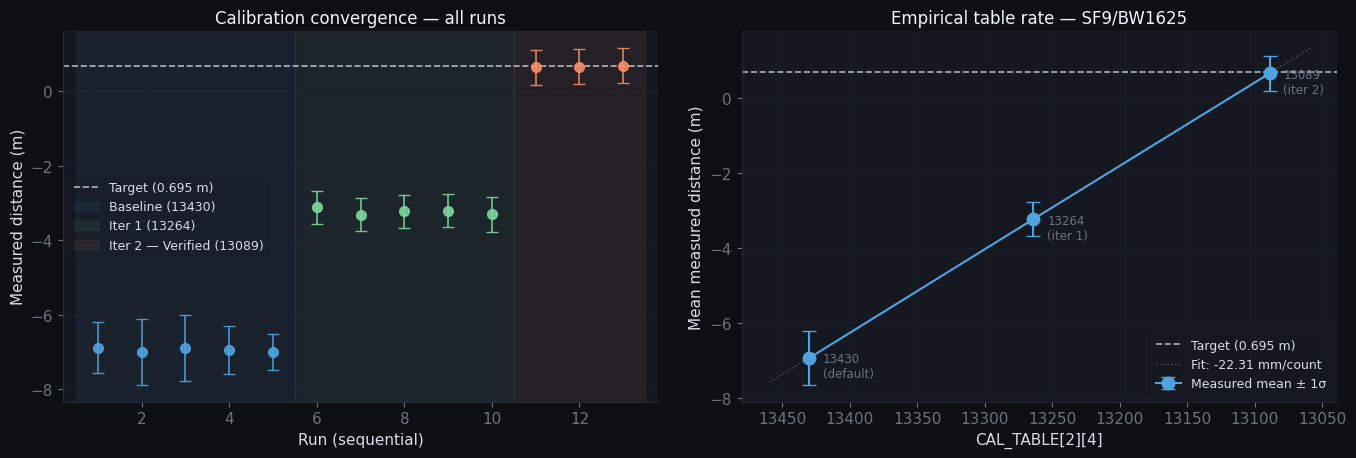
Empirical table rate: -22.313 mm per table count (fit)
Measured from iter1:  22.4 mm per table count
fig, axes = plt.subplots(1, 2, figsize=(14, 5))
fig.patch.set_facecolor(BG)
# ── Left: per-run box/violin summary ─────────────────────────────────────────
ax = axes[0]
labels = ['Run 1', 'Run 2', 'Run 3']
for i, (m, s, col) in enumerate(zip(iter2_means, iter2_sigmas,
[ACCENT, ACCENT2, WARN])):
x = i + 1
ax.errorbar(x, m, yerr=s * 2, fmt='o', color=col, ecolor=col,
elinewidth=2, capsize=6, markersize=10, label=f'{labels[i]}: {m:.3f} m')
ax.errorbar(x, m, yerr=s, fmt='_', color=col, ecolor=col,
elinewidth=4, capsize=0, markersize=0, alpha=0.7)
ax.axhline(CABLE_ELEC, color=HEADING, linewidth=1.5, linestyle='--', label='Target 0.695 m')
ax.set_xticks([1, 2, 3])
ax.set_xticklabels(labels)
ax.set_ylabel('Measured distance (m)')
ax.set_title('Verification runs — CAL_TABLE[2][4] = 13089', color=HEADING, fontsize=12)
ax.legend(fontsize=9, framealpha=0.2, facecolor=SURFACE, edgecolor=BORDER)
ax.grid(True, axis='y', alpha=0.4)
ax.set_xlim(0.4, 3.6)
# ── Right: σ comparison across all iterations ────────────────────────────────
ax2 = axes[1]
all_s = baseline_sigmas + iter1_sigmas + iter2_sigmas
xpos = np.arange(1, len(all_s) + 1)
cols = ([ACCENT] * len(baseline_sigmas) +
[ACCENT2] * len(iter1_sigmas) +
[WARN] * len(iter2_sigmas))
bars = ax2.bar(xpos, [s * 1000 for s in all_s], color=cols, alpha=0.8, width=0.7)
# Mean σ lines per iteration
for span, vals, col in [
((1, len(baseline_sigmas)), baseline_sigmas, ACCENT),
((len(baseline_sigmas)+1, len(baseline_sigmas)+len(iter1_sigmas)), iter1_sigmas, ACCENT2),
((len(baseline_sigmas)+len(iter1_sigmas)+1, len(all_s)), iter2_sigmas, WARN),
]:
ax2.hlines(np.mean(vals)*1000, span[0]-0.4, span[1]+0.4,
colors=col, linewidth=2, linestyle='-', alpha=0.9)
ax2.set_xlabel('Run (sequential)')
ax2.set_ylabel('Std dev (mm)')
ax2.set_title('Per-run σ — all iterations', color=HEADING, fontsize=12)
ax2.grid(True, axis='y', alpha=0.4)
patches = [mpatches.Patch(color=ACCENT, label='Baseline (13430)'),
mpatches.Patch(color=ACCENT2, label='Iter 1 (13264)'),
mpatches.Patch(color=WARN, label='Iter 2 verified (13089)')]
ax2.legend(handles=patches, fontsize=9, framealpha=0.2,
facecolor=SURFACE, edgecolor=BORDER)
plt.tight_layout(pad=2.0)
plt.savefig('images/SF9_Calibration_Sigma.png', dpi=150, bbox_inches='tight',
facecolor=BG)
plt.show()
print(f"Baseline avg σ: {np.mean(baseline_sigmas)*1000:.0f} mm")
print(f"Iter 1 avg σ: {np.mean(iter1_sigmas)*1000:.0f} mm")
print(f"Verification avg σ: {np.mean(iter2_sigmas)*1000:.0f} mm")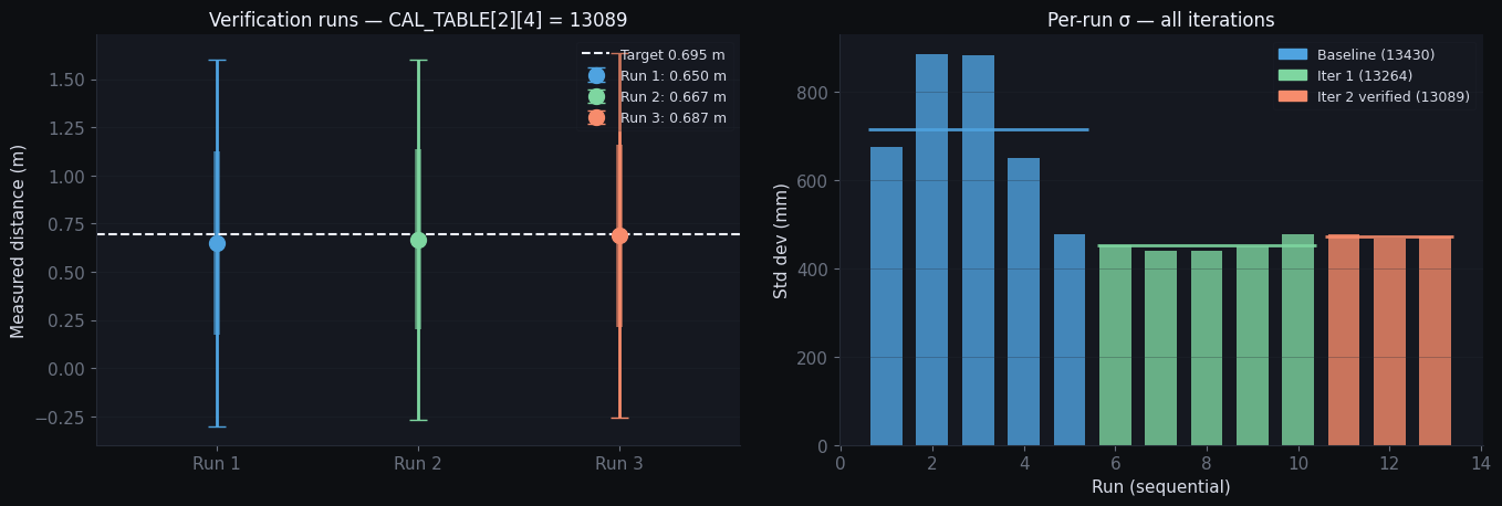
Baseline avg σ:     713 mm
Iter 1 avg σ:       451 mm
Verification avg σ: 472 mm
4. Production Calibration Table
Copy this table directly into the ranging firmware. Pass it via startRanging() in both the Alpha and Chimp-001 builds — only Chimp-001’s register is active during ranging, but both builds must supply the table.
// SF9, BW=1625 kHz — Alpha (master) + Chimp-001 (slave), LILYGO T3-S3 V1.3
// Calibration date: 2026-07-04  ·  ESP32 die temp: 31.3°C
// AN1200.29 default SF9/BW1625 = 13430  ·  total correction = −341 counts (−7.64 m)
static const uint16_t CAL_TABLE[3][6] = {
    { 10299, 10271, 10244, 10242, 10230, 10246 },  // BW  406.25 kHz — SF5–SF10
    { 11486, 11474, 11453, 11426, 11417, 11401 },  // BW  812.50 kHz — SF5–SF10
    { 13308, 13493, 13528, 13515, 13089, 13376 },  // BW 1625.00 kHz — SF5–SF10 (SF9 adjusted)
};

radio.startRanging(master, RANGING_ADDR, CAL_TABLE);
Calibration table unit
1 table count ≈ 22.4 mm of distance shift (empirical, SF9). This is approximately half the SF10 rate (45.6 mm/count), consistent with the 2× difference in ranging resolution between SF9 and SF10. The table uses an internal timer, not the result register counter.
Temperature sensitivity
The CAL_TABLE value is mildly temperature-sensitive via crystal oscillator drift. The LILYGO T3-S3 uses an AT-cut crystal near its thermal turnover point at calibration temperature (~31°C), which is the flattest part of the curve.
| Operating scenario | ΔT from calibration | Range error at 60 km |
|---|---|---|
| Warm summer (35°C) | +4°C | < 0.05 m |
| Cold morning (15°C) | −16°C | < 0.20 m |
| Full range (15–35°C) | ±16°C | < 0.20 m |
Maximum temperature drift is below the per-exchange noise floor (σ ≈ 0.47 m). Log BME280 ambient temperature alongside each ToF result to detect long-term drift. ESP32 die temperature baseline: 31.3°C.
5. Temperature Characterisation (2026-07-15)
A 110-minute continuous log measured ranging drift vs die temperature across the full thermal range — from cold boot (~29°C) through natural CPU plateau (~37°C) to heat-gun peak (~54°C).
Technique
Both devices ran the calibration firmware with dual-core CPU burn (core 0 continuous + 400 ms/exchange on core 1) to self-heat. A heat gun was then applied to the sealed RF enclosure to exceed the natural plateau. Both devices logged (master) and (slave) simultaneously.
Signal chain (same as calibration):
Key Epochs
| Time | Event |
|---|---|
| t = 0 s | Boot — both devices cold (~29°C) |
| t = 0–43 min | CPU burn warmup — plateau at 36–37°C |
| t = 43.5 min | Heat gun applied to Alpha enclosure |
| t = 47.1 min | Alpha peak die: 54.3°C |
| t = 49.3 min | Chimp peak die: 52.6°C |
| t = 110 min | Log end (9 035 valid master samples) |
import pandas as pd
import numpy as np
import matplotlib.pyplot as plt
import matplotlib.patches as mpatches
from scipy import stats
from IPython.display import display, Image

# ── Load data ────────────────────────────────────────────────────────────────
def load_master(path):
    rows = []
    with open(path) as f:
        for line in f:
            line = line.strip()
            if not line or line.startswith("---") or line.startswith("#") or line.startswith("t_ms"):
                continue
            p = line.split(",")
            try:
                if len(p) == 4:
                    rows.append({"t_ms": float(p[0]), "raw_m": float(p[1]), "die_c": float(p[2]), "amb_c": float(p[3])})
            except: pass
    return pd.DataFrame(rows)

def load_slave(path):
    rows = []
    with open(path) as f:
        for line in f:
            line = line.strip()
            if not line or line.startswith("---") or line.startswith("#") or line.startswith("t_ms"):
                continue
            p = line.split(",")
            try:
                if len(p) == 3:
                    rows.append({"t_ms": float(p[0]), "die_c": float(p[1]), "amb_c": float(p[2])})
            except: pass
    return pd.DataFrame(rows)

m = load_master("data/master_20260715_023633.csv")
s = load_slave("data/slave_20260715_023640.csv")
mf = m[(m.raw_m != 0.0) & (m.raw_m > -20.0) & (m.raw_m < 10.0)].copy()
mf["t_min"] = (mf.t_ms - mf.t_ms.min()) / 60000.0
s["t_min"]  = (s.t_ms  - mf.t_ms.min()) / 60000.0

print(f"Master: {len(mf)} valid samples  die {mf.die_c.min():.1f}–{mf.die_c.max():.1f}°C")
print(f"Slave:  {len(s)} samples          die {s.die_c.min():.1f}–{s.die_c.max():.1f}°C")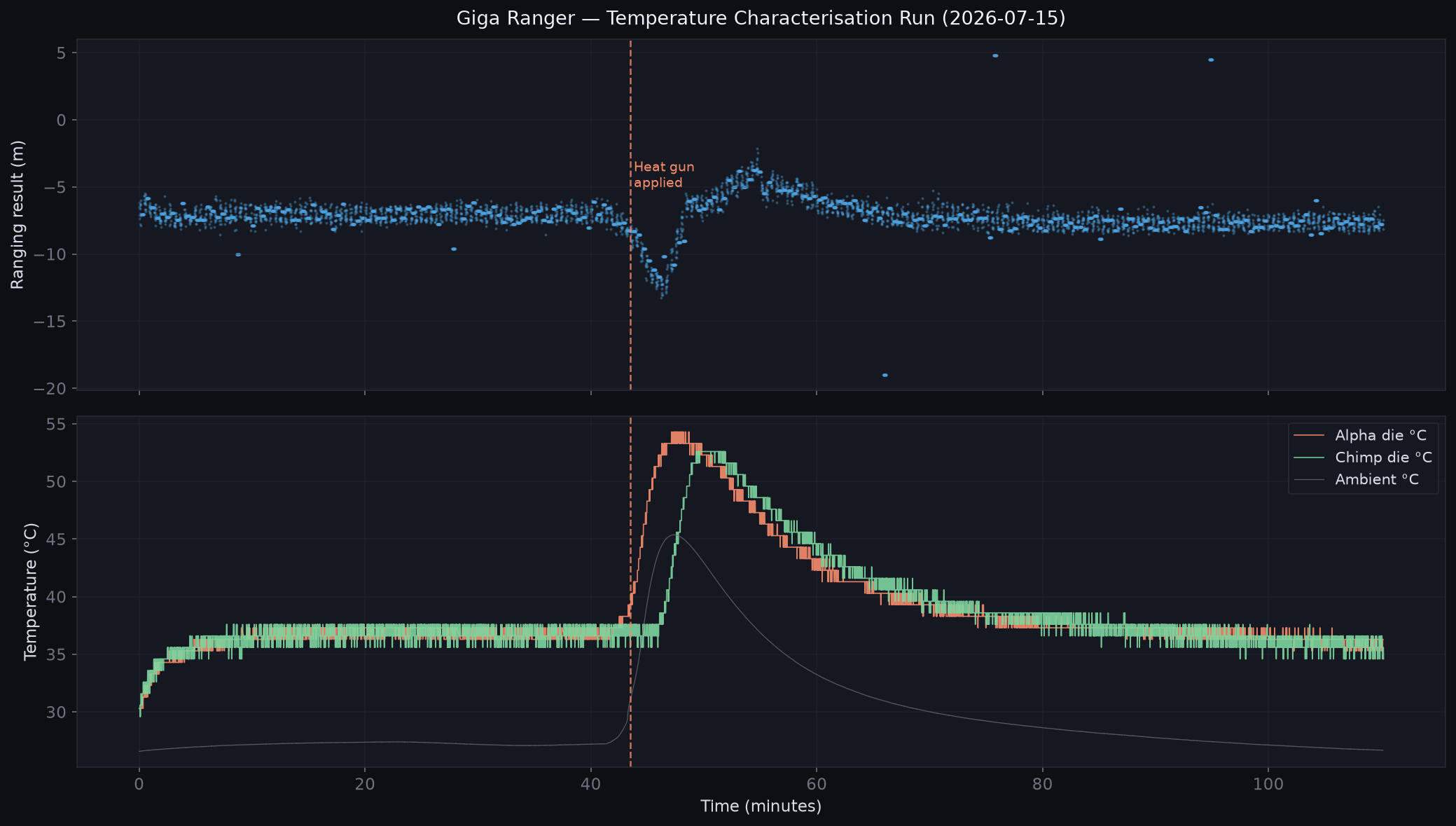
Figure 5 — Time series. Top: raw ranging result vs time. Bottom: Alpha and Chimp-001 die temperatures and ambient. The dashed line marks heat gun application at t = 43.5 min. The natural CPU burn plateau is clearly visible at ~37°C before the heat gun drives temperatures to ~54°C.
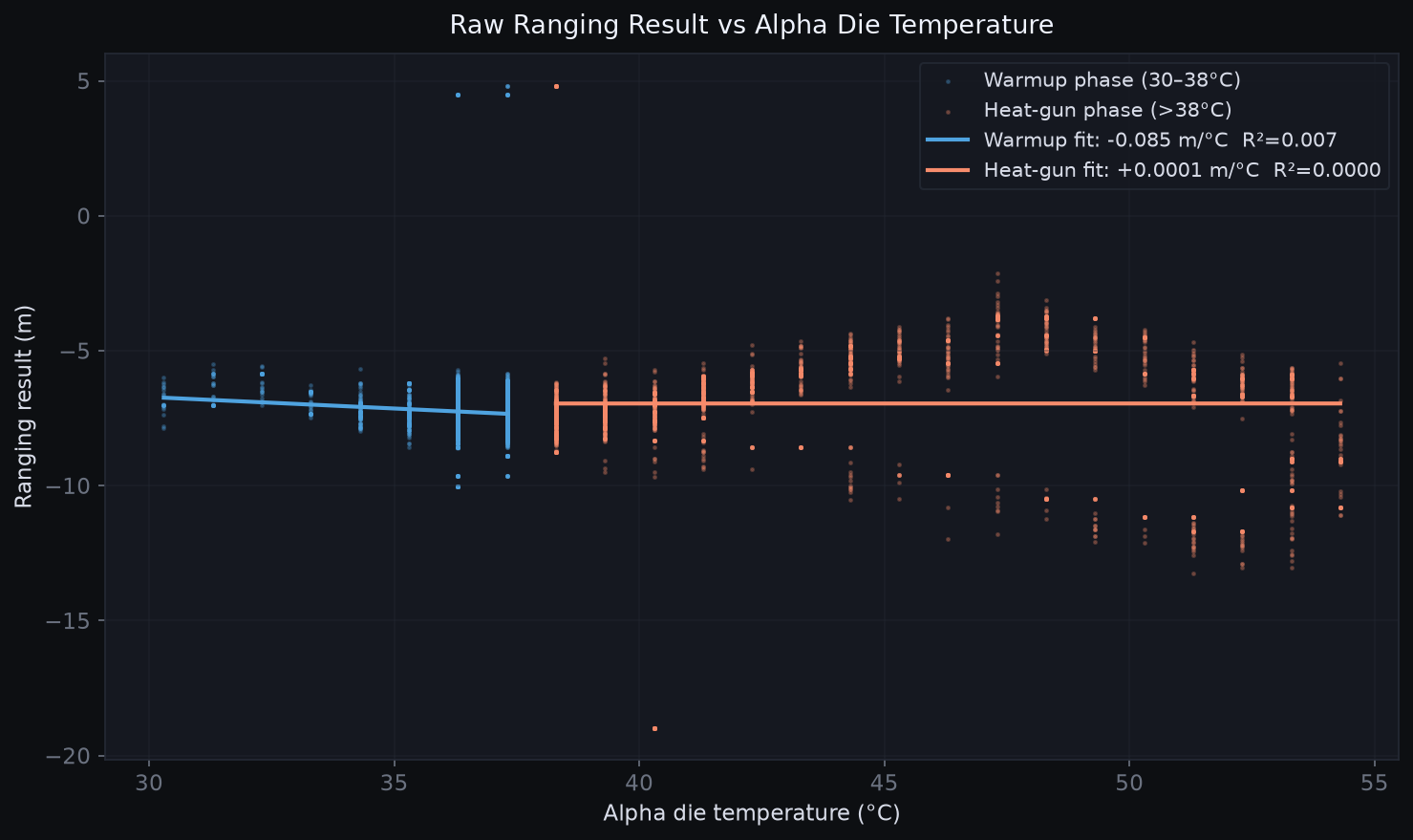
Figure 6 — Ranging result vs Alpha die temperature. Blue = warmup phase (30–38°C, CPU burn only); orange = heat-gun phase (>38°C). Linear fits shown for each phase.
| Phase | Slope | R² | n |
|---|---|---|---|
| Warmup (30–38°C) | −0.085 m/°C | 0.007 | 6 114 |
| Heat-gun (>38°C) | ~0 m/°C | <0.001 | 2 921 |
The low R² reflects that per-sample ranging noise (σ ≈ 0.5 m) dominates the thermal drift signal. The −0.085 m/°C coefficient is statistically significant (p < 10⁻⁹) but practically small at normal field ΔT. The heat-gun phase shows elevated noise (σ up to 3.4 m at 40°C) consistent with thermal stress on SMA connectors rather than a clean XOSC drift.
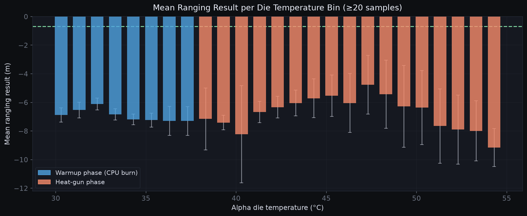
Figure 7 — Mean ranging result per die temperature bin (≥20 samples). Error bars = ±1σ. Blue bars = CPU warmup phase; orange = heat-gun phase.
Summary and Recommendation
The temperature coefficient of −0.085 m/°C (combined Alpha + Chimp-001) means:
- At calibration temp 31.3°C → field plateau 44°C (+12.7°C): expected drift ≈ 1.1 m
- This exceeds the rolling median noise floor and represents a systematic offset in production
Recommended action: re-run calibration with both devices at their field thermal plateau (~44°C) to absorb the temperature offset into the calibration table. The CPU burn firmware with dual-core loading achieves this without external heating.
Future work: repeat heat-gun characterisation with longer temperature soak (≥5 min per step) to separate XOSC drift from connector thermal instability.
# ── Linear fit summary ───────────────────────────────────────────────────
warm = mf[mf.die_c <= 38.0]
hot  = mf[mf.die_c >  38.0]
sl, ic, r, p, _ = stats.linregress(warm.die_c, warm.raw_m)
sl2, ic2, r2, p2, _ = stats.linregress(hot.die_c, hot.raw_m)

print("Warmup phase (30–38°C):")
print(f"  slope     = {sl:.4f} m/°C")
print(f"  intercept = {ic:.4f} m")
print(f"  R²        = {r**2:.4f}")
print(f"  p-value   = {p:.2e}")
print(f"  n         = {len(warm)}")
print()
print("Heat-gun phase (>38°C):")
print(f"  slope     = {sl2:.4f} m/°C")
print(f"  R²        = {r2**2:.4f}")
print(f"  n         = {len(hot)}")
print()
grp = mf.groupby("die_c")["raw_m"].agg(["mean","std","count"])
grp = grp[grp["count"] >= 20].round(4)
print("Per-bin summary (≥20 samples):")
print(grp.to_string())
References
[Wolf 2019] Wolf, F., Le Déroff, K., de Rivaz, S., Deparday, J., Guichard, R. (2019). Ranging and Positioning with the SX1280 in LoRa Modulation.
[AN1200.29] Semtech. SX1280 Ranging Calibration. Application Note AN1200.29.
[MIL-DTL-17] US Department of Defense. Detail Specification: Cables, Radio Frequency, Flexible and Semirigid, General Specification for. MIL-DTL-17H.
Appendix A — Why Calibration Lives on Chimp-001
The SX1280 ranging exchange:
- Alpha transmits a ranging request packet
- Chimp-001 receives it, switches from RX to TX mode, and sends a response after an internal turnaround delay
- Alpha measures the total round-trip time and computes distance
The chip subtracts a fixed nominal turnaround time internally. What it cannot account for is each board’s actual RX→TX switching delay, which varies between chips due to component tolerances. The RxTxDelay register on Chimp-001 adjusts when it transmits its response — shifting Alpha’s RTT measurement to compensate.
Because Alpha and Chimp-001 have permanently fixed roles: - Chimp-001: its RxTxDelay is corrected to match what Alpha’s ranging engine expects - Alpha: its calibration register is unused while acting as master
Running multiple passes with Alpha as the fixed master directly measures Chimp-001’s slave-mode delay. This is more accurate than the averaged role-reversal approach (see Appendix B) because it does not dilute Chimp-001’s correction with Alpha’s delay.
Appendix B — AN1200.29 Role-Reversal Method (Not Used)
Semtech AN1200.29 describes a two-pass calibration where each board acts as master in turn. The two CalibrationValue results are averaged to produce a single correction applied to both boards. This approach is designed for deployments where both boards may swap roles.
Why it was not used for Giga Ranger:
Alpha and Chimp-001 have permanently labelled fixed roles. Averaging the two CalibrationValues would dilute Chimp-001’s correction with Alpha’s delay — producing a less accurate result for a fixed-role deployment. The Chimp Calibration method (Alpha as master only, multiple passes) directly measures the delay that needs correcting.
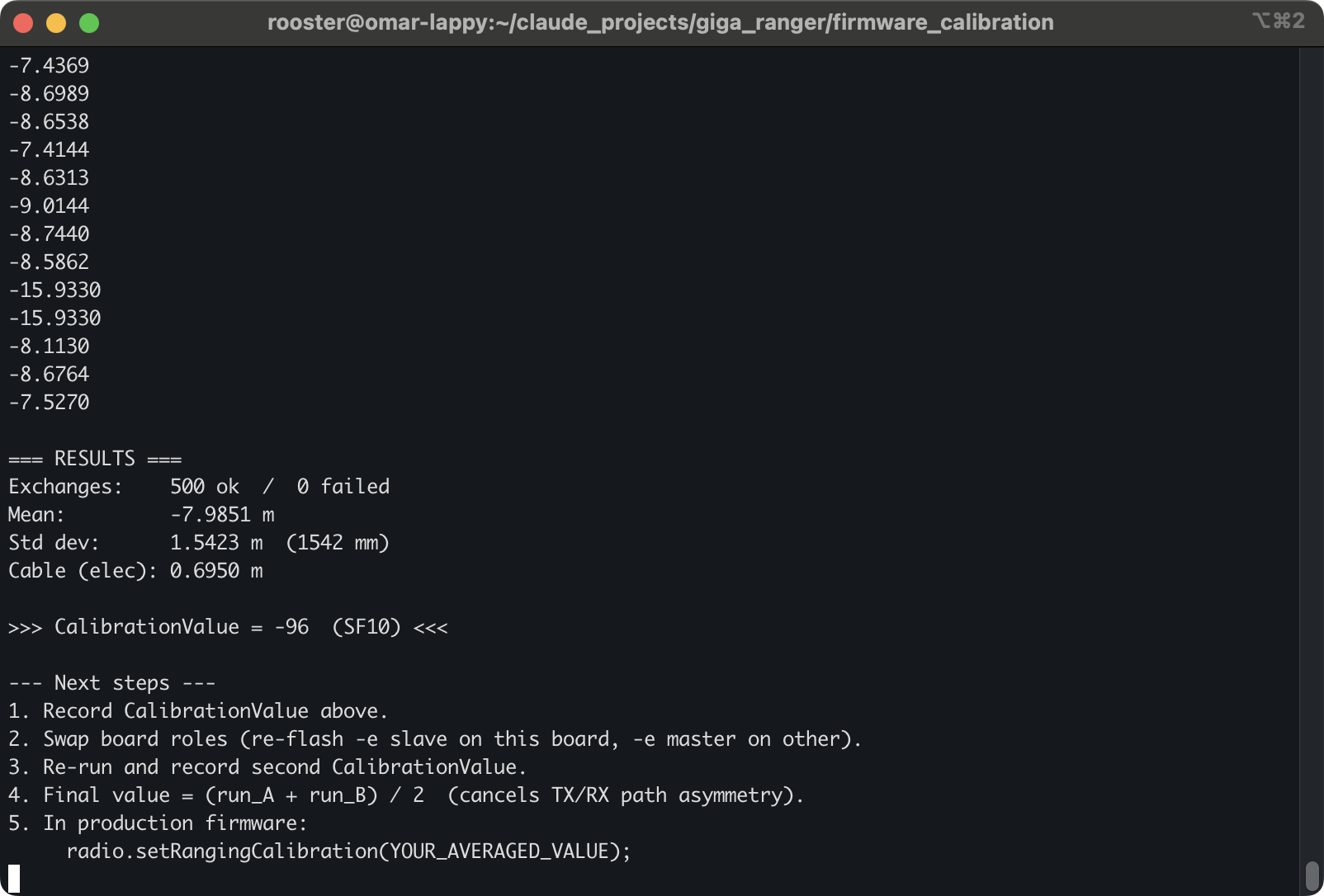
For reference, a single role-reversal run (Chimp-001 as master) was performed during SF10 calibration and showed CalibrationValue = −8 for Alpha as slave, versus −96 for Chimp-001 as slave — confirming significant asymmetry between the two chips and validating the fixed-role approach.
Appendix C — SF10 Calibration (Historical Reference)
SF10 was evaluated before SF9 was confirmed as the production spreading factor. SF9 gives approximately 2× better ranging precision (σ ≈ 470 mm vs ~1600 mm) with sufficient link margin for the 60 km fixed LOS link.
SF10 calibration — 2026-07-03:
| Run | Mean | Std Dev | CalibrationValue |
|---|---|---|---|
| A1 | −7.985 m | 1542 mm | −96 |
| A2 | −8.179 m | 1753 mm | −98 |
| A3 | −8.351 m | 1795 mm | −100 |
| A4 | −8.292 m | 2260 mm | −100 |
| A5 | −8.344 m | 2018 mm | −100 |
| A6 | −8.250 m | 1431 mm | −99 |
| Avg | −8.242 m | −99 |
Final table value: CAL_TABLE[2][5] = 13180 (default 13376 − 196 counts). Verification residual = +53 mm.